
The demonstrator presents a system for detection of faults in industrial drives and their state of health estimation. Data coming from the inverter and vibrations sensors are analysed using ANN and information on detected and classified faults is used for purposes of predictive maintenance. In some cases, control can be adapted to mitigate the fault in real-time, which allows further operation of the drive in degraded mode (fail-operational drive). Application of the designed system results in the drive having higher reliability and availability, which is important for highly and fully automated production systems.
Research Focus
| Diagnostics of production machines components – drives, rotating machines |
Target
| For companies dealing with highly reliable and available actuators in various industrial (and automotive/airspace) use-cases. |
Demonstrator description
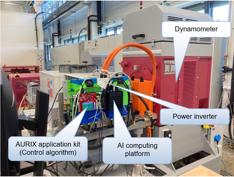
The demonstrator uses the dynamometer connected with dual three-phase PMS motor with the possibility of fault injection. The motor is controlled with 6-phases power inverter. Its control board is based on AURIX 2G microcontroller which is connected to nVIDIA Jetson Xavier platform. The purpose of the demonstrator is to analyse different faults in motor and the inverter enabling models’ development, dataset generation, development of methods for fault detection, either classical ones or AI based. The demonstrator also serves for the development of diagnostic algorithms from vibration measurements.
Hardware
The demonstrator consists of experimental dual there-phase PMS motor with piezoelectric vibration sensors and microphone, power inverter with additional powerful computing platform, and fault insertion unit for fault emulation.
Multiphase Motor with the Terminal Block
The motor is designed to allow operation during the faults (fail-operational). For this reason, a two-times-three-phase structure was chosen. Mutual inductance between individual sub-systems of the motor is low, allowing the fault to be isolated in one three phase sub-system, while the healthy (fault-free) part of the motor can continue to operate. To achieve this behaviour, the field weakening index is also crucial, and for this motor, its value is less than one.
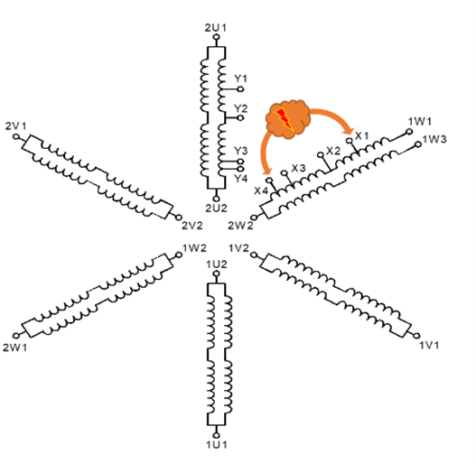
Motor has prepared many windings taps so various types and severities of the interturn short-circuit faults can be emulated.

Six-Phase Inverter
The power inverter used in the demonstrator was designed to allow the connection of two three-phase motors or one dual three phase motor (see Figure 3). It is composed from two interconnected three-phase Infineon hybrid kits. The control of the inverter is realized with the microcontroller Infineon TC297. It has six cores, enabling the implementation of not only the control algorithm but also various algorithms for motor state monitoring. Higher number of cores enables also the implementation of simple algorithms based on artificial neural networks directly into the microcontroller.
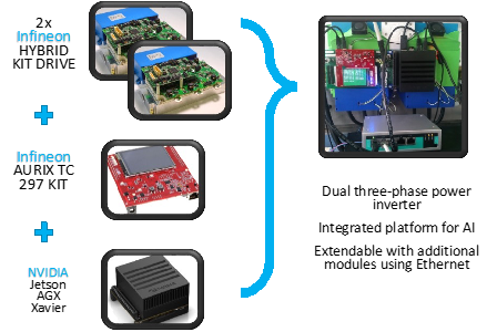
The power inverter is joined with an nVIDIA Jetson Xavier unit, which is connected to the microcontroller via an Ethernet network. This additional unit allows the implementation and testing of complex algorithms based on artificial neural networks or other machine learning techniques.
Fault Insertion Unit
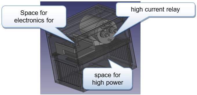
Various interturn short-circuits are emulated using the fault insertion unit (Figure 4). The fault insertion unit is capable of repeatedly creating shorts at precisely defined time intervals by using a parallel combination of a relay and a power thyristor. This unit allows the creation of a short circuit with a value of up to 500 A rms.
Sensors for Measurement of Mechanical Quantities
Additional sensors for measurement of mechanical quantities (as shown on Figure 2) can be classical piezoelectric accelerometers (in this case PCB type JTLD352C04) and a microphone (Brüel&Kjaer Type 4958) or a specialized complex sensing device containing several MEMS transducers for different quantities in one industrial housing. Structure of such complex sensor for diagnostics based on non-electrical quantities measurement sensor designed and implemented by us is shown on Figure 5 and except vibration and noise transducers it contains a specialized transducer for ultrasonic emission measurement (acoustic surface wave acquisition) and a temperature sensor (inside MEMS low frequency accelerometer). All data processing tasks shown on Figure 5 is done in one ARM Cortex M4 processor from ST Microelectronics.
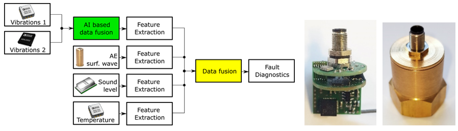
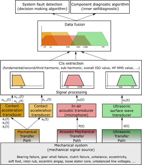
Mechanically generated movement (e.g., vibration of the motor caused by a failure) is transferred from the measured structure to the surrounding environment and sensed by appropriate transducer. Each transfer path has its own transfer function defining parameters of coupling of the sensor to the base structure. Three different mechanical quantities are acquired – acceleration a(t) sensed by a MEMS accelerometer(s), sound pressure p(t) sensed by a MEMS microphone and displacement d(t) sensed by an acoustic emission (AE) sensing element. Electrical signal from all elements is led to the internal signal processing block and output processed data are available in digital form on the output interface of the sensor (CAN bus or RS-485).
The complex diagnostic sensor is available also as a digital twin designed in MATLAB at a level of individual transducers integrated in the whole device. The applied model structure for each of the internal transducers is shown on Figure 6.
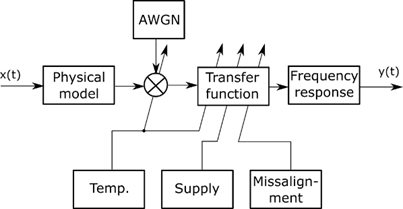
Block named “Physical model” represents the natural resonance of the physical sensing element (MEMS cantilever, MEMS membrane). Additive white Gaussian noise is afterwards added to the signal. The amount of noise is temperature dependent. Transfer function represents the internal gain of the sensor (its sensitivity) and is affected by the temperature of the sensor, supply voltage (since the sensitivity is ratiometric value), and also by the misalignment of the mechanical system in case of multi-axis sensing element. The last block named “Frequency response” provides frequency dependent shaping of the signal and represents the working bandwidth of the sensing element. Since all the aforementioned parameters can be easily found in the datasheet of any sensing element (like accelerometers, gyroscopes, MEMS microphones, piezo elements etc.), this model prototype can be used for any sensor modelling.
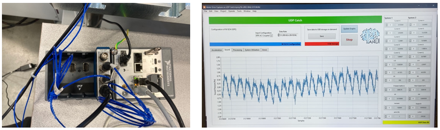
Output signals (analog and/or digital) from the sensor(s) of non-electrical quantities measurements are connected to NI CompactRIO signal processing platform serving as interfacing and additional data pre-processing unit for mechanical sensing and is also connected to the power inverter using Ethernet for interchanging electrical/mechanical data. A picture of the cRIO platform connected to the sensors with analogue output is show on Figure 7 left. Acquired signal waveforms from different sensors and digital electrical data from power invertor can be reviewed using LabVIEW application running on cRIO, as shown on Figure 7 right.
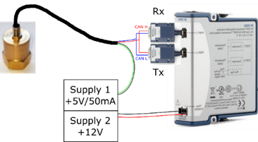
In case of using only the complex diagnostic sensor for acquisition of all non-electrical quantities, its connection to the CompactRIO platform is realized using CAN interface card NI XNET as shown on Figure 8.
Software Framework
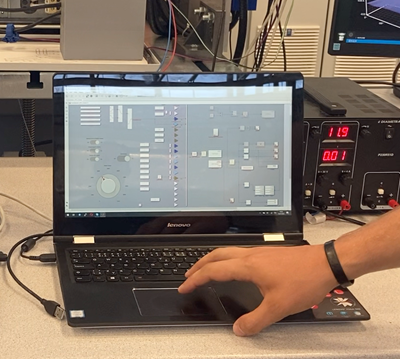
High level control and monitoring application runs in MATLAB Simulink. It is capable to control dynamometer, tested motor, CompactRIO platform, nVIDIA Jetson, and fault insertion unit. The photo can be seen in Fig. 9.
Involvement of AI Tools
The prepared hardware platform allows the use of a program for the processor or the utilization of parallel computing using GPU with the use of an additional computing module.
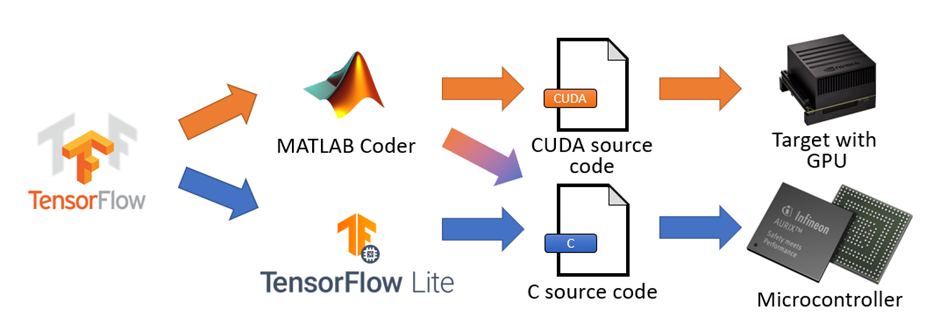
For this reason, software tools were chosen to allow efficient implementation of artificial neural networks, either into the microcontroller or the GPU. The neural network is designed and trained using the TensorFlow environment. Prepared neural networks can be exported in various formats. The next step in deploying prepared ANN into target HW is loading ANN into the MATLAB environment. MATLAB allows the generation of CUDA code or C/C++ code. MATLAB does not support all layers available in the TensorFlow environment, so ANN needs to be prepared with respect this fact. MATLAB can generate CUDA source code using almost all supported layers. However, the possibility of generating C/C++ code is significantly reduced, and only basic layers can be used. This property is not a problem because large neural networks with advanced layers, such as convolutional layers, recurrent layers, or LSTM layers, cannot be implemented in microcontrollers because of memory demands. Another alternative for ANN deploying is using the TensorFlow Lite for microcontrollers. In this case, the neural network is converted into a basic format and implemented together with the TensorFlow lite for microcontrollers. TensorFlow lite for the microcontrollers requires a 32-bit target platform.
Framework for AI based Inter-Turn Short-Circuit Fault Detection Utilizing Mechanical Quantities
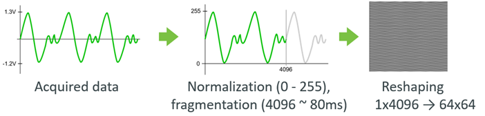
Data pre-processing of vibration/noise signals is performed in cRIO platform using LabVIEW application. It contains normalization of data and its transformation into 2D images. Complete pre-processing flow of data can be seen on Figure 11.
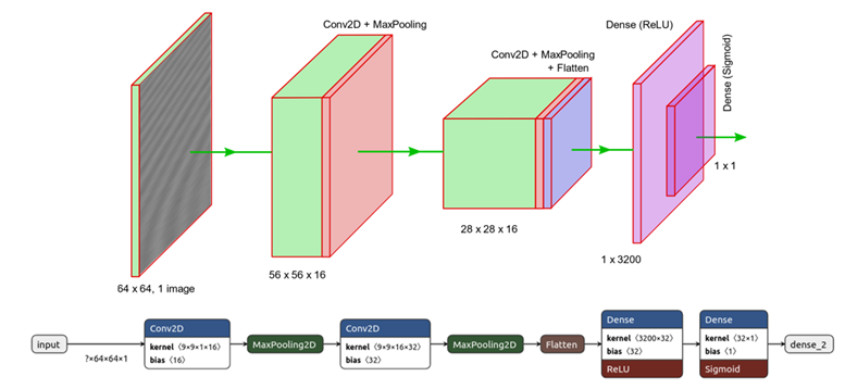
These images serve as an input to the 2C CNN designed in Keras environment, where the structure of the network was modelled, trained, and evaluated. The network structure is on Figure 12 and contains two convolutional layers and two dense layers. Neural network has one neuron in the output layer with the binary output, where its value of zero represents healthy state of the motor and a value of one represents induced fault of a motor.
At the Edge Condition Indicators Calculation, Sensor Data Fusion and Bearing Faults Classification
The internal signal processing block inside the complex diagnostic sensor performs condition indicators (CI) calculation based on the fixed algorithms implementation inside the block. Data fusion block afterwards ensures appropriate combination of all signals into one optimal input to the decision block, where it can contain not only system fault detection block ensuring detection of mechanical and electrical faults of a diagnosed system, e.g., unbalance, bearing failures, short circuits in the rotor windings etc., but also inner self-diagnostic block ensuring internal diagnostics of the sensing device and its health status. The complete signal and data processing flow applied in the complex diagnostic sensor is on Figure 14.
Based on our knowledge about the ability of specific condition indicator to contain information about the specific mechatronic system fault, there were created a list of them and connected to the physical sensing domain (e.g., quantity) where their evaluation is the most beneficial.
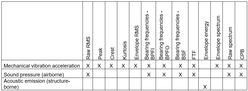
From the table it can be seen that vibration measurement is still a key domain for evaluating the machine health status. All measured and calculated values are trended and normalized using reference value stored at the beginning of the machine life cycle or at the beginning of the sensing procedure, thus the CI value is greater than or equal to one, where a value of “one” means the good condition and any higher value means certain level of faulty condition. In practice, it is quite hard to set the appropriate limits, therefore, the exact threshold values have to be found on empiric basis, measurements, or previous knowledge about the machine.
Combination of a powerful microcontroller with set of transducers in one complex diagnostic sensor gives us a possibility to deploy AI based identification approaches inside the device itself and provide classified data directly to a superior controller. Unfortunately, the low power microcontroller STM32L4 used in the sensor allows us to implement only shallow neural networks.
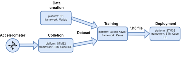
Therefore, also the learning phase of neural network process was performed on another more powerful platform (Jetson Xavier AGX or GeForce RTX 2080 Ti inside PC) and the resulted model (both architecture and parameters) was stored to a standard *.h5 file. This file can be read with the development environment of the microcontroller who compiles the model to C code. Specific development environment for STM32 processors is STM32CubeIDE, which was also used for C code generation in this case. The applicability of neural networks for vibration data classification were tested using the development workflow described on Figure 16 and the implemented ANN model designed in MATLAB is on Figure 17.
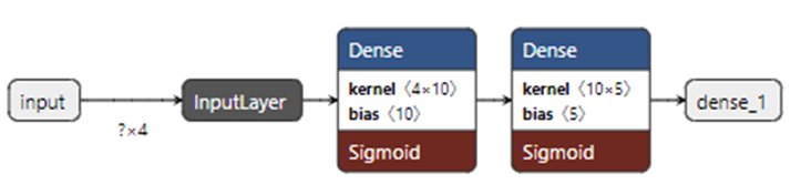
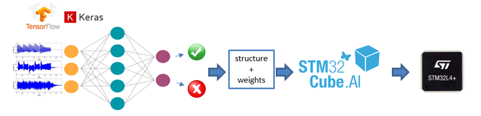
In case of direct modelling and designing of ANN in Keras environment, the workflow for deployment of the ANNs into the complex sensing device (at the edge device) is on Figure 35.
Communication Platform
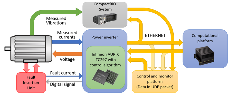
The basic communication takes place between the control microprocessor and the nVIDIA computing unit. The hardware is designed to enable communication between these two modules either through SPI communication or via Ethernet. For the final demonstrator, communication through Ethernet was used, where the control microcontroller sends all real-time data from the control algorithm as a UDP packets using broadcast. These data are utilized in the nVIDIA computing platform for the condition monitoring algorithm. nVIDIA processes this data and sends information about any detected faults back to the control process. Real-time data are aso used in CompactRio platform. Simultaneously, all data is collected by the computer that controls and monitors the entire system (control and monitoring platform). The data can be later used to improve detection algorithms. The full topology of the demonstrator can be seen in Figure 19.
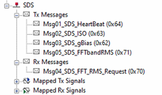
Real-time data from electrical system are also used in NI CompactRIO platform, where Ethernet UDP packets transferred from AURIX platform each 100 µs (10 kHz) as a broadcast message and transmits all electrical data (phase currents), speed of the motor and an applied torque by the dynamometer represented mainly as 4-bytes single precision float number is received. Connection of signals from classical sensors for mechanical quantities measurement to cRIO platform is realized using analog IEPE interface, thus no communication protocol is utilized. Connection of the complex diagnostic sensor (SDS – smart diagnostic sensor) to the cRIO platform is based on CAN communication where all possible messages provided by the sensor can be described in CAN interface database file. As an example, five CAN messages can be implemented inside the sensor. Three of them are cyclic and generated by the sensor, one message is generated by the supervised system (e.g., cRIO) and creates a request for FFT band value calculation, and one message is the response from SDS with the FFT band value. A structure of the messages can be seen in the following Figure 20. Thanks to detailed *.dbc database, which defines all the signals, scaling factors, units, data types, ranges etc. the implementation is very simple and straightforward. The types and structures of CAN messages can be modified through updating firmware of the main MCU of the sensor.
Scenario Description (Applications)
Demonstrator shows the possibility to detect various depths of the interturn short circuit from the real-time measured control parameters and vibrations measured by vibration sensors. Interturn short-circuit with given severity is generated using the fault insertion unit (FIU). Fault severity is configured by connection of the FIU to the motor. Fault can be emulated in two different phases. Each of these phases is located in different sub-system, so faults detection algorithm can be validated very precisely.
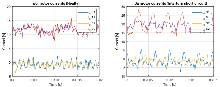
In Figure 22, we can examine the phase currents recalculated into dq coordinates for both the healthy and faulty states. Notably, the currents of the impaired sub-system display noticeable distortion, particularly in the form of a second harmonic component. This observed distortion is consistent with the outcomes derived from mathematical analyses specifically tailored to this type of fault. The distinctive characteristics in the damaged sub-system currents, as evidenced by the prominent second harmonic, underscore the utility of employing dq coordinates for effectively diagnosing and analyzing motor faults.
These signals can be used as input variables into some types of the ANN. Long sequences can be used in convolutional neural networks. In this case large number of convolutional filters is required to detect the fault under various operation conditions. The alternative comes from using recurrent neural networks, which can consider information extracted from previous samples or conversion of the data into a more appropriate format.
In Figure 23, the low pass filtered magnitudes of the motor currents in αβ coordinates can be seen. In an ideal scenario with the motor and power inverter operating steadily, these magnitudes should remain constant and unaffected by the motor’s electrical angle. Nevertheless, both healthy and faulty waveforms exhibit the presence of a sixth harmonic component. This particular harmonic component is primarily a result of the dead-time effect. The examination of an inter-turn faults reveals a notable augmentation in the second harmonic component, distinctly observable in the αβ current magnitude waveform. However, what is more important, second harmonics is not time depended in this case.
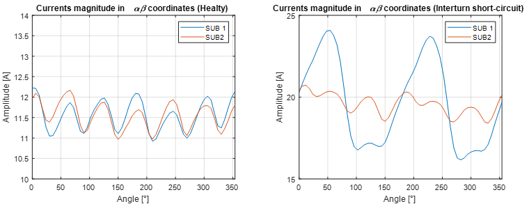
The presented data are formatted as fixed-size vectors, serving as input variables for convolutional neural networks or simpler multi-layer perceptron neural networks. Both types of neural networks underwent training using measured data. The demonstrator effectively showcases and validates the feasibility of employing these approaches to detect inter-turn short circuits in PMS motors.
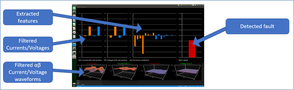
The resulting program responsible for monitoring the motor’s condition is implemented on the Jetson Xavier. The final application during testing can be seen in Figure 24. The visualization includes displaying inputs to the neural network as well as the outcome of fault detection, indicated by a colour changes.
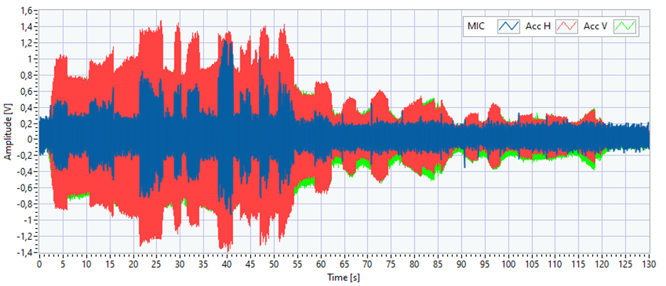
Additionally to the previous approach focusing on fault detection in the electrical motor using electrical quantities as inputs to the artificial neural network, there has been also implemented, tested and validated an approach involving measurement of mechanical quantities to detect faults in the electrical part of the motor. In this case, measured quantities were vibration and acoustic signals measured on or close to the motor. Example waveforms obtained during one test run is on Figure 25.
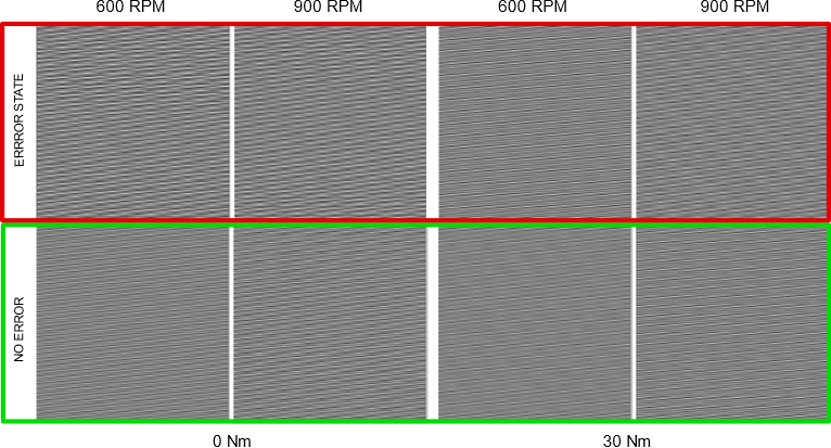
These quantities as time series were transformed to 2D images and these 2D data serve as inputs to the convolutional neural network. For information, several 2D images of vibration data representing healthy and faulty states of the motor during different operating conditions (torque, speed) can be seen on Figure 26.
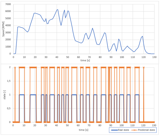
Applied speed profile and corresponding induced and predicted faults during the test are shown on Figure 27. Predicted state of the motor is multiplied twice for better visibility.
Time delay of the prediction of the fault is defined by the delay of the processing in the neural network and is equal to the value of the 80 ms. This time corresponds to duration of the input signal which represents one image frame with the size of 64×64 data points. As it can be seen from induced and predicted waveforms on Figure 27, the two profiles are almost identical and total classification accuracy is 99.1 %. There are few occasions when the classification is not ideal. Mostly the classification problem is caused by the non-ideal image size which is a trade-off between the minimized delay of the prediction and the duration of the input signal.
Regarding bearing fault analysis, it is hard to obtain real data on running machine, therefore vibration signals potentially measured on faulty bearing were generated artificially using vibration exciter and fault signal generator as can be seen on.
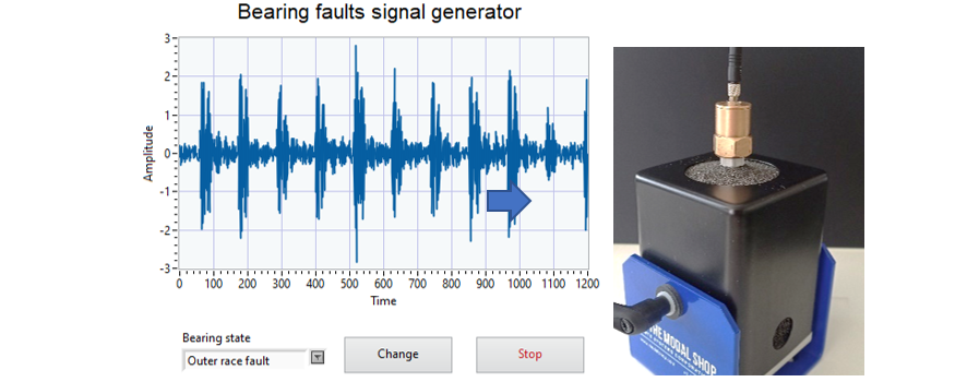
Four bearing health states were used for classification – healthy bearing and several types of bearing damage.
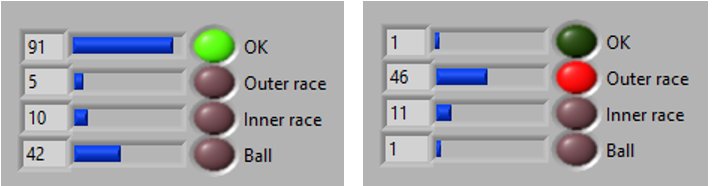
Outcome of the classification of bearing faults performed directly inside the diagnostic sensor and visualized in the connected superior system (e.g., process monitoring computer) is on Figure 46. There can be seen not only identified type of fault, but also its probability.
List of Used Modules and Realized Applications
| Module Name | Description | Application |
| AI based classifier of interturn shorts using electrical quantities | CNN designed in Keras/TensorFlow and using MATLAB coder transferred to CUDA source code for nVIDIA Jetson AI/GPU platform and/or using TensorFlow Lite directly into the AURIX microcontroller. | Real-time diagnostics of production machines components – drives. |
| AI based classifier of interturn shorts using mechanical quantities | 2D CNN designed in Keras environment and deployed on high performance computer connected to the pre-processing unit represented by NI CompactRIO platform. | Diagnostics of production machines components – drives, in specific working conditions. |
| AI based classifier of mechanical wear and bearing faults damage using mechanical quantities | Dense neural network designed in MATLAB environment and deployed directly in smart sensor. | Diagnostics of production machines – rotating machines. |